This is a walk through the front half of a manuscript I’ve been working on, When Does Unrolling Help Flow Matching? (full PDF). The short version: training a flow-matching model the way it is actually sampled — unrolling the solver and backpropagating through it — is the obvious fix for a real problem, but it’s the wrong default. Analyzing why is the interesting part, because it lands on a clean result: consistency and shortcut models fall out of unrolled flow matching once you apply a gradient-variance argument.
The gap nobody trains for
Flow Matching / Conditional Flow Matching (CFM) learn a velocity field whose ODE transports noise \(x_1\) to data \(x_0\) along a straight path \(x_t = t\,x_1 + (1-t)\,x_0\). Training is simulation-free: you regress the network onto the marginal velocity at independently sampled times \(t\), always evaluated on the true interpolation path.
But inference does something categorically different — it integrates the learned field with a discrete solver over \([0,1]\). A small directional error at step \(t\) nudges the sample off the data manifold and compounds at the next step. That discretization drift (a form of exposure bias) never appears in the training signal, and the network is never asked to correct a state it produced itself.
Unrolling: the obvious fix, and the twist
The natural remedy — call it Windowed Trajectory Flow Matching (WT-FM): unroll the discrete solver for a window of \(L\) steps, feed each step its own previous prediction, and backpropagate the terminal trajectory error through the intermediate generated states (Backpropagation Through Time, BPTT). Now training sees the same compounding error that inference does.
The twist: run naively — full BPTT on the terminal error, which turns out to equal the \(k\)-step negative ELBO — this does not beat well-tuned single-step training. The contribution isn’t the objective; it’s what its analysis reveals.
The main result: consistency & shortcut models fall out
Grounding the unrolled loss in the \(k\)-step ELBO and expanding it exposes a weighted single-step FM term plus trajectory cross-terms:
\[\mathcal{L}_{k\text{-step}} = \mathbb{E}\!\left[\sum_i \|\hat v^i-v^i\|^2\,w_i \;+\; \sum_{i\neq j}(\hat v^i-v^i)^{\top}(\hat v^j-v^j)\,w_{ij}\right]\]Those cross-terms are the only place BPTT couples steps — they’re what let an error at step \(i\) be cancelled by a compensating error at step \(j\) (self-correction). But their gradient variance compounds as \((\mathrm{Var}(x_0\mid x_t))^{L}\), which is exactly what makes full BPTT fragile. So a gradient-variance argument motivates dropping them — and dropping them is precisely what detaching the teacher between steps does. Via a summation-by-parts / Cauchy–Schwarz bound, what remains is:
\[\tfrac{1}{K^2 dt^2}\,\|E_k\|^2 \;\lesssim\; \underbrace{\|\hat v^1 - v^1\|^2}_{\text{single-step FM (anchor)}} \;+\; \Big(\tfrac{K-1}{K}\Big)^2\,\underbrace{\mathbb{E}_i\,\|\hat v^i - \hat v^{i-1}\|^2}_{\text{self-consistency}}\]which is — up to weighting — consistency models and shortcut models. The framing I like: these aren’t separate heuristics; they’re the variance-anchored limit of unrolled flow matching.
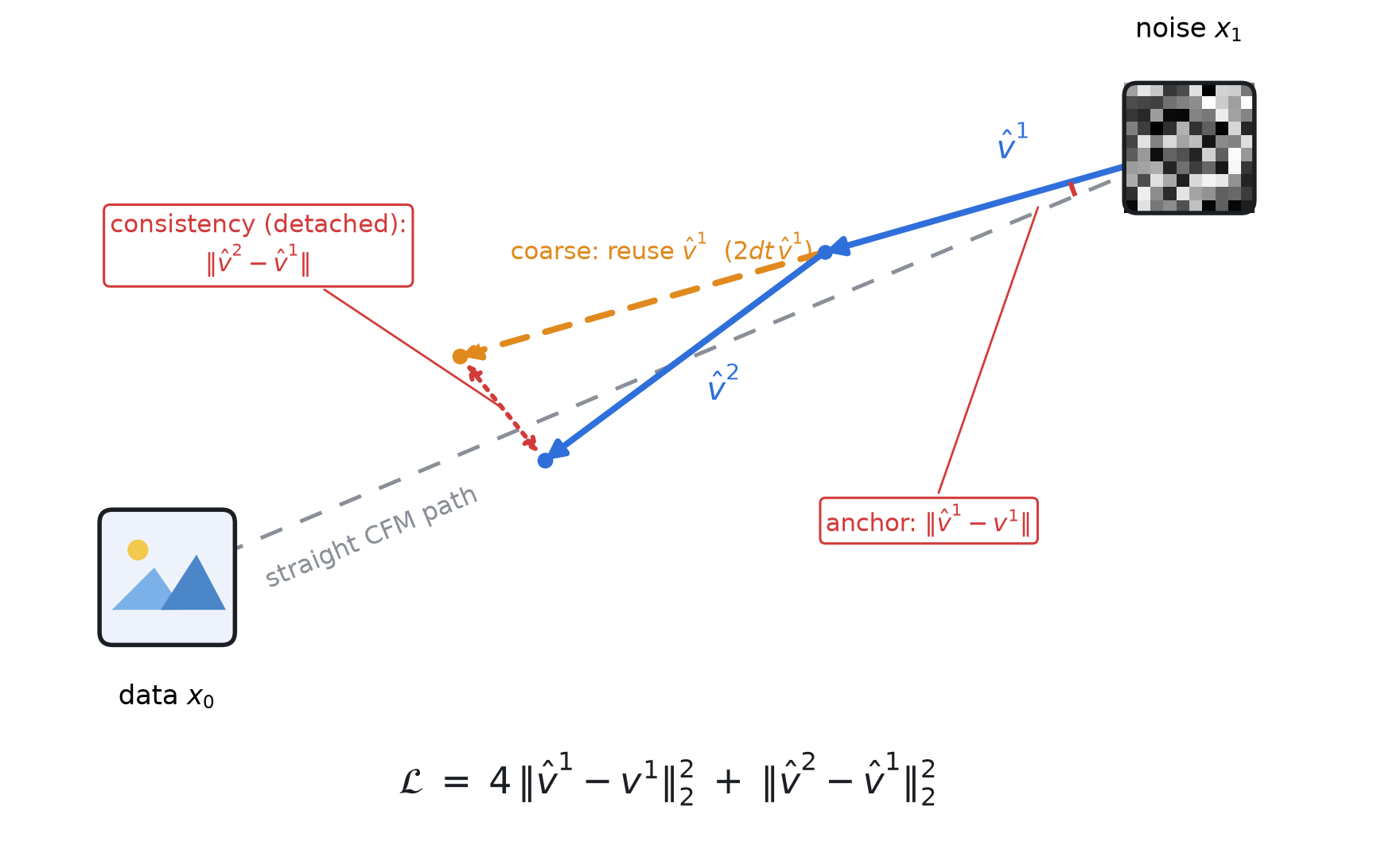
From noise \(x_1\), the true straight CFM path (gray) reaches data \(x_0\). The shared first step \(\hat v^1\) (blue); the coarse step reuses it for a doubled jump (\(2dt\,\hat v^1\), dashed orange); the fine trajectory re-evaluates and turns with \(\hat v^2\). Dropping the cross-terms leaves an anchor term \(\|\hat v^1-v^1\|\) (single-step FM) plus a detached consistency term \(\|\hat v^2-\hat v^1\|\), giving \(\mathcal{L}=4\|\hat v^1-v^1\|^2+\|\hat v^2-\hat v^1\|^2\).
The nice part is how literal this is in code. In
synthetic_testbench/losses.py
the whole reduction is one function:
def Shortcut_BPTT_Loss(pred_vs, target_v, detach):
    preds = torch.stack(pred_vs)                        # [W, B, D]
    original_err = F.mse_loss(preds[0], target_v)       # anchor = single-step FM
    if detach:
        teacher_targets = (preds[1:].mean(0)).detach()  # detach -> frozen self-teacher
    else:
        teacher_targets = preds[1:].mean(0)             # full BPTT (keeps the graph)
    self_consistency_err = F.mse_loss(preds[0], teacher_targets)
    return 0.8 * original_err + 0.2 * self_consistency_err   # ~4:1 (the Taylor weight)
The detach flag is the whole story: with it on, you get the consistency/shortcut
form; with it off, full BPTT. And the 0.8 / 0.2 split is the same 4:1 weighting
that shows up in the figure’s loss.
Why the field parametrization beats \(\hat x_0\)
There are two ways to parametrize the network: output the velocity/field directly, or output a clean-data estimate \(\hat x_0\) (with the velocity implicit via \(\hat v=(\hat x_0-x_t)/t\)). Under unrolling, their transition Jacobians differ decisively:
\[\mathbf{T}^{\text{field}} = \mathbf{I}+dt\,\mathbf{J}_{\hat v} \qquad\qquad \mathbf{T}^{\hat x_0} = \Big(1-\tfrac{dt}{t}\Big)\mathbf{I}+\tfrac{dt}{t}\,\mathbf{J}_{\hat x_0}\]The field Jacobian is a near-identity (\(dt\ll 1\)) — numerically inert but
stable. The \(\hat x_0\) loss and Jacobian both carry a \(1/t\) factor
(in code, the 1/(t**2 + eps) weight in target_loss), which blows the
gradient up near the data manifold (\(t\to 0\)). At matched training loss,
\(\hat x_0\) carries roughly \(3\times\) the mean gradient norm with far larger
swings across noise levels:
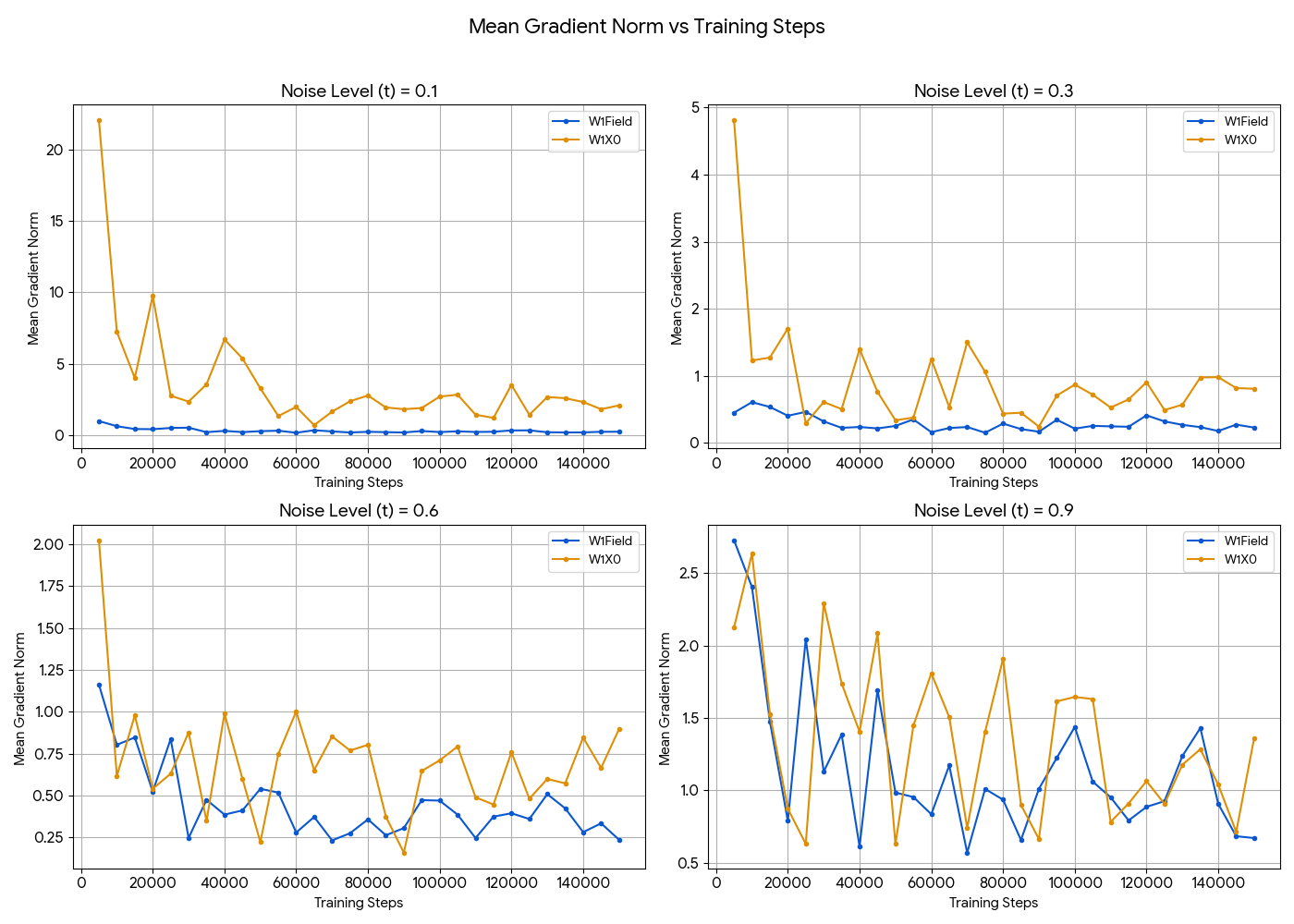
Mean gradient norm vs training steps at four noise levels. Field (blue) stays flat and small; \(\hat x_0\) (orange) spikes — up to ~22 at \(t{=}0.1\) vs the field’s ~0.3 — and stays noisier everywhere. On the 2D manifolds \(\hat x_0\) is 130–690% worse in Wasserstein-1; on CelebA-\(64^2\) its FID trails field.
Why minibatch OT: collapse the conditional variance
The remaining instability is statistical. With independent couplings, \(\mathrm{Var}(x_0\mid x_t)\) grows exponentially as \(t\to 1\), the single-step gradient variance is proportional to it, and under unrolling it compounds multiplicatively across the \(L\) steps. Minibatch optimal-transport couplings re-pair source and target within each batch, straightening the interpolant and collapsing that conditional variance — the single most consistent stabilizer across every setting I tried.
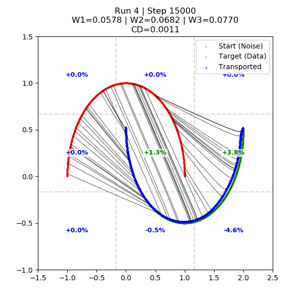
OT-coupled transport on two-moons at 15k steps: noise (red) to data (green), the transported samples (blue) following near-straight coupling lines, with \(W_1/W_2/W_3 \approx 0.058 / 0.068 / 0.077\).
Bottom line
Unrolled flow matching is best understood not as an end in itself, but as the
derivation that anchors consistency- and shortcut-style training. The recipe
that falls out is: minibatch OT + field parametrization + dropped cross-terms
(anchored consistency). The same objective carries over from the 2D testbench
to CelebA-\(64^2\) (via celeba_ddpm/looped_model.py over a Karras-UNet
DDPM backbone), where field again beats \(\hat x_0\) on FID.
Manuscript: When Does Unrolling Help Flow Matching? (PDF).
Code: Windowed-trajectory-flow-matching
(synthetic_testbench/ for the 2D experiments, celeba_ddpm/ for CelebA).