Paper (arXiv:2610.17375) · Code · LLaDA-8B-Instruct-PIG · Nemotron-Labs-Diffusion-3B-PIG
With Anton Xue, Sanjay Shakkottai and Sujay Sanghavi (UT Austin).
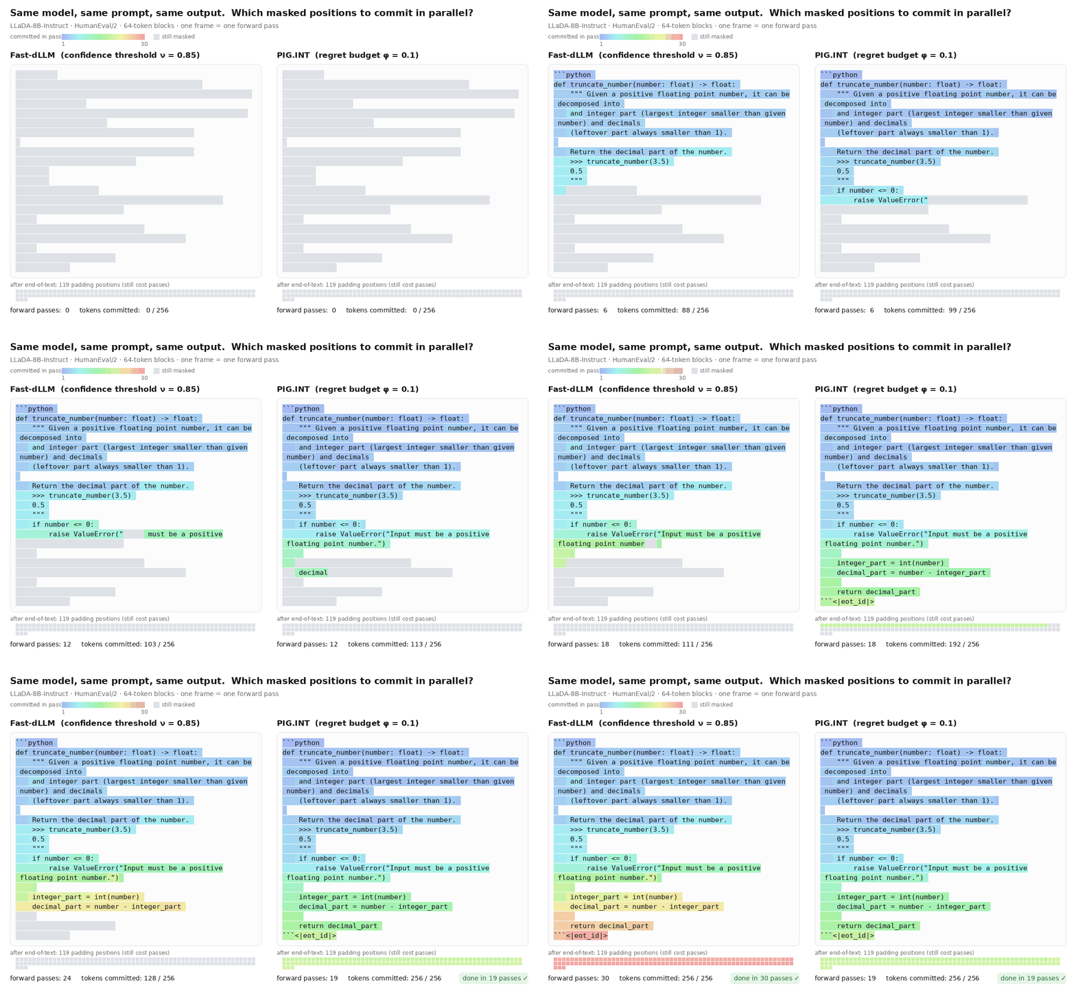
Two decodes of the same prompt by the same model (LLaDA-8B-Instruct, 64-token blocks). Every frame is one forward pass; a token’s colour is the pass that committed it. Left: Fast-dLLM, which commits every token above a confidence threshold. Right: PIG.INT, which commits as many tokens as its predicted inconsistency budget allows. Both produce the identical program. One needs 30 passes, the other 19. Over all 164 HumanEval problems at this geometry the two operating points sit at 7.2 and 10.1 tokens per forward pass, at 36% and 34% pass@1 (Wilson 95% intervals of about seven points).
At a glance
- Same model, same outputs, fewer forward passes. PIG changes only which masked positions get committed together. The backbone is frozen and the tokens it produces are the ones it would have produced anyway.
- Almost free at inference. The adapter has about 2M parameters and costs under 0.1% of the arithmetic of one forward pass; the whole selection step adds about 13 ms per round on a shared H100, an upper bound.
- Cheap to train, trained once. One harvest of exact finite differences (26 GPU hours on a single H100) and about an hour to fit the adapter, on a small training-side mixture. The same adapter then serves every benchmark, budget and block geometry, including MMLU, which it never saw.
- Up to 1.7× the tokens per forward pass of Fast-dLLM at matched accuracy on LLaDA, 1.4× over Nemotron’s native decoder, and up to 28 more accuracy points at the baseline’s fastest settings.
The problem: tokens committed together cannot see each other
A masked diffusion language model predicts every masked position from the same canvas in a single forward pass. That is where its speed comes from: you can reveal many positions per pass instead of one. It is also where the trouble comes from. Positions committed in the same pass never get to condition on each other. If one slot could be “dog” or “cat” and another “barks” or “meows”, each prediction is fine on its own, and committing them together can still produce “dog meows”.
Decoding one token at a time avoids this, because the canvas is updated after every commit. It is the slow oracle: it respects the model’s own joint distribution, and it throws away all the parallelism.
Existing parallel decoders pick positions using two kinds of signal. Confidence methods, with Fast-dLLM as the standard baseline, commit whatever the model is sure about. Dependence methods such as DAPD avoid committing positions that look coupled, for instance through attention. Both are proxies for the thing we actually care about.
A different question
Take a candidate set of positions the decoder is about to commit in parallel, in some order. Ask: would the model have written the same tokens if it had decoded those positions one at a time, in that order? Any disagreement is what we call sequential–parallel inconsistency. It is not confidence and it is not dependence; it is the error that parallelism actually introduces, measured against the sequential trajectory of the same model.
\[\textbf{sequential:}\;\; \mathbf{x}_t \xrightarrow{x^*_{s_1}} \mathbf{x}_{t+1} \xrightarrow{x^*_{s_2}} \cdots \xrightarrow{x^*_{s_k}} \mathbf{x}_{t+k} \qquad \textbf{parallel:}\;\; \mathbf{x}_t \Rightarrow \{\hat{x}_{s_1},\dots,\hat{x}_{s_k}\}\]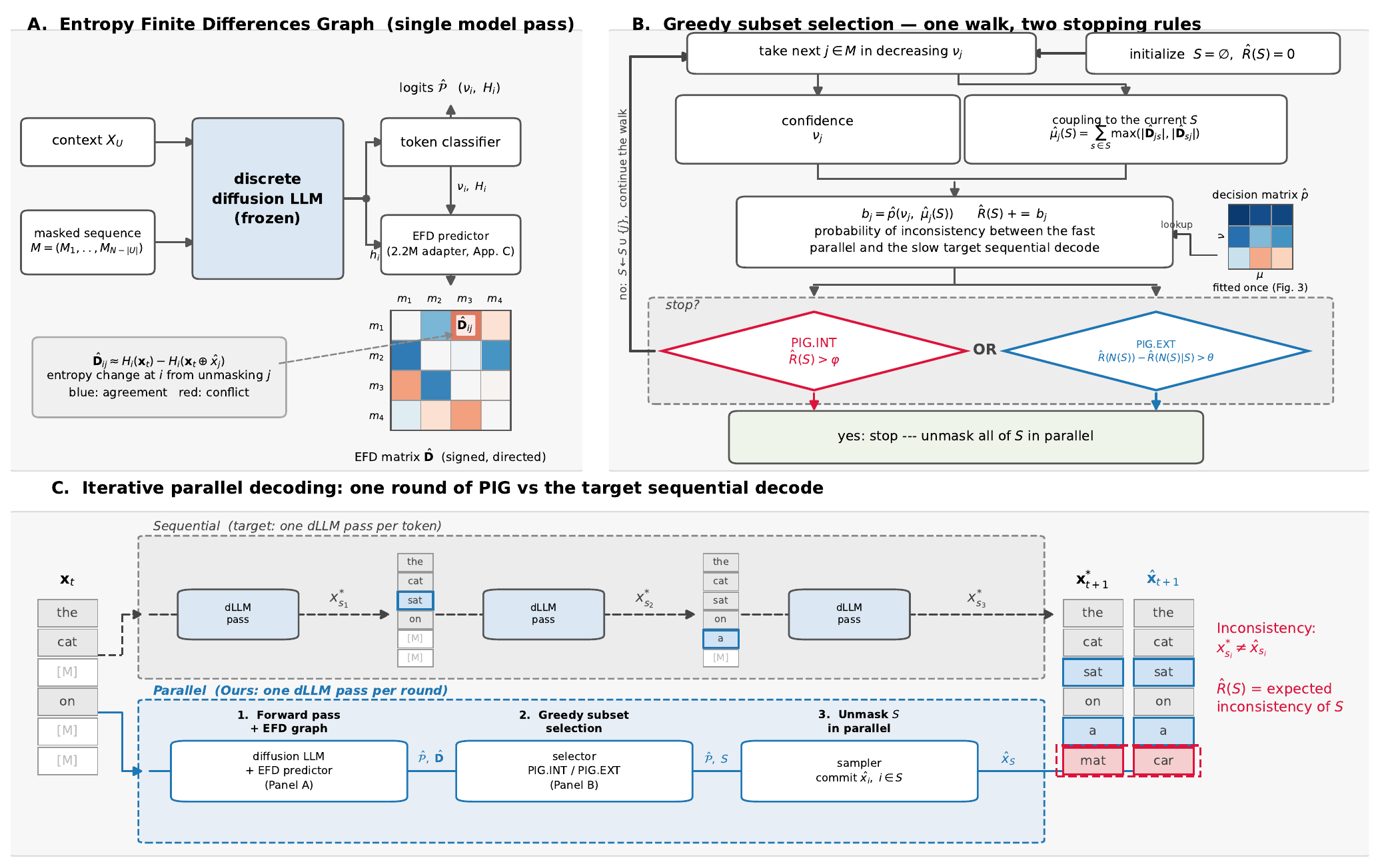
(A) A small predictor on the frozen model estimates how committing one position would change the entropy at every other. (B) Candidates are admitted in decreasing confidence until the predicted regret passes a budget. (C) One parallel round against its sequential target: “the cat sat on a mat” versus “the cat sat on a car” is the inconsistency we want to avoid.
If this inconsistency were known before committing, parallel decoding would be a plain selection problem: commit as many positions as you can while the predicted disagreement stays small. The catch is that measuring it exactly means replaying the candidates one at a time, which is the slow decode we were trying to avoid.
You do not have to replay
It turns out the replay is predictable from the forward pass you already have. Committing position \(j\) changes the model’s uncertainty at every other position \(i\). We write that change as an entropy finite difference,
\[\mathbf{D}_{ij} = H_i(\mathbf{x}_t) - H_i(\mathbf{x}_t \oplus \hat{x}_j),\]signed: positive when committing \(j\) would make \(i\) more certain, negative when it would make \(i\) less certain (the two predictions are in tension). The Finite Differences Estimator (FDE), a lightweight adapter on the frozen backbone with about 2M parameters and under 0.1% of a forward pass in arithmetic, predicts the whole matrix \(\hat{\mathbf{D}}\) from the hidden states of one pass. On held-out benchmarks it reaches a correlation of about 0.8 per edge and 0.9 on the aggregate statistics the decoder actually consumes.
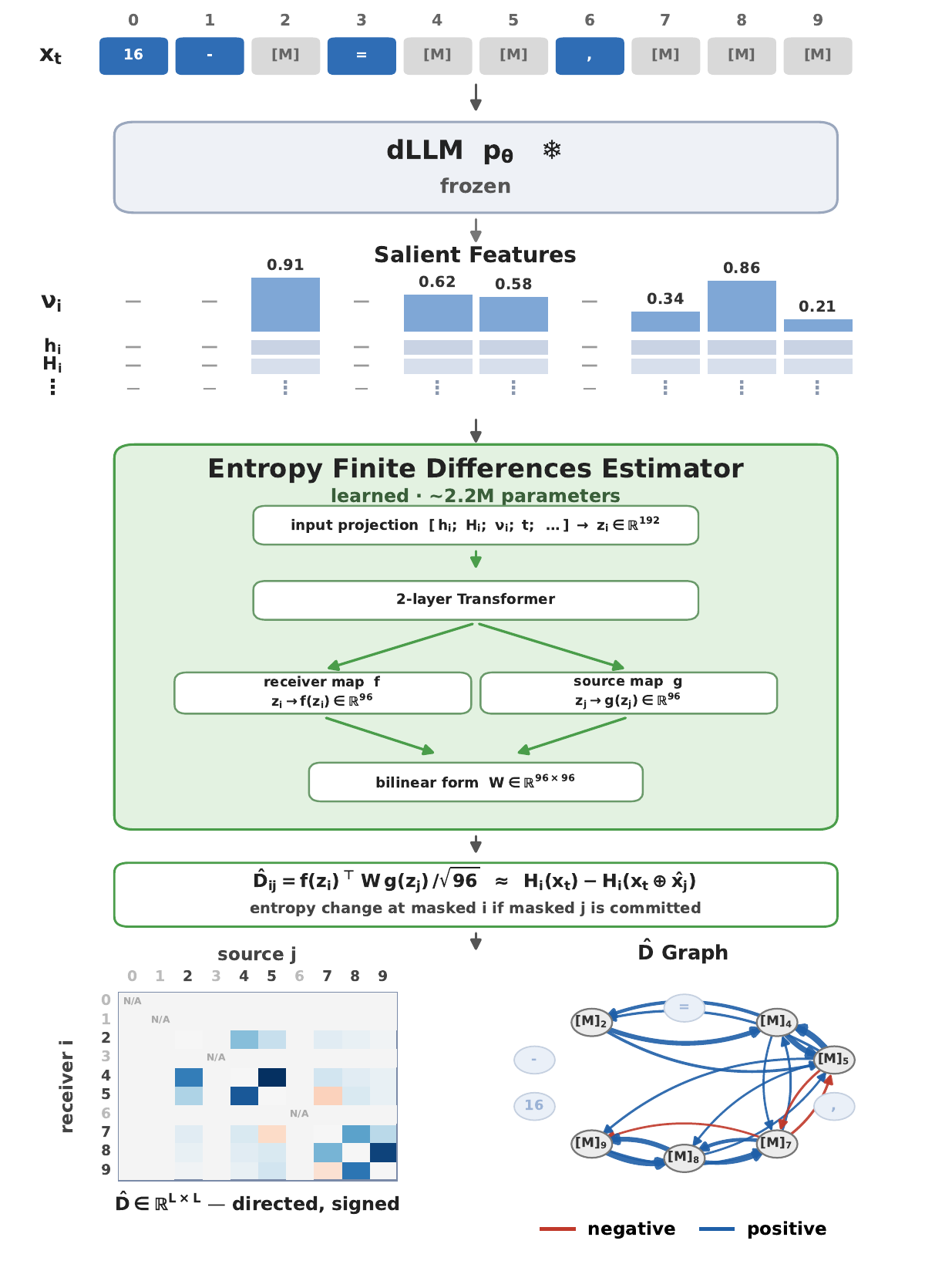
One forward pass of the frozen model gives per-position features (confidence, entropy, hidden states); the Finite Differences Estimator turns them into \(\hat{\mathbf{D}}\) for the whole canvas with one matrix product.
Here is what the matrix looks like on a real pass of the decode above, for the 24 most confident candidates in the block:
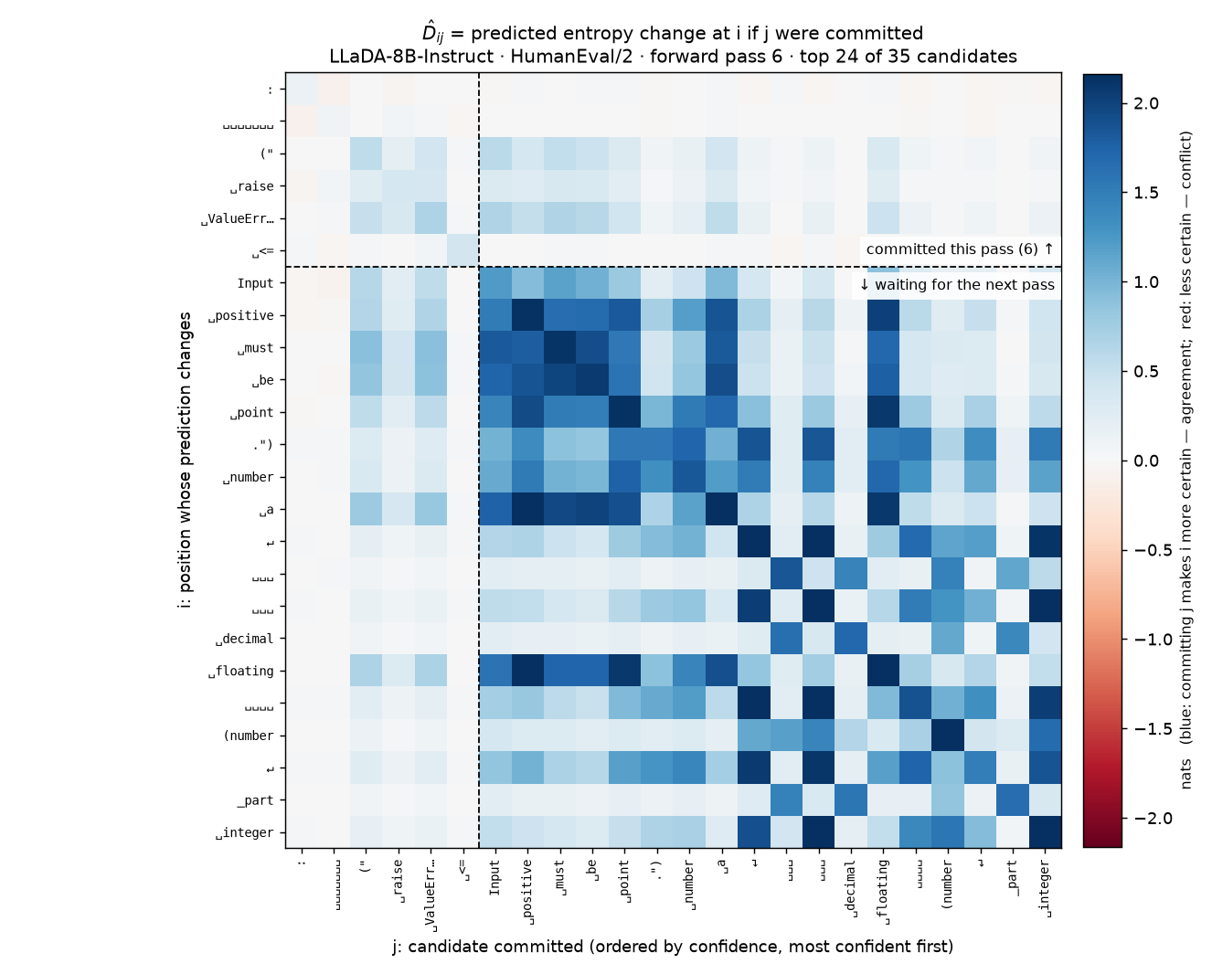
Rows are positions whose prediction would change, columns are the candidates that could be committed; blue means committing the column would make the row more certain, red that it would unsettle it. The dashed lines separate what PIG.INT committed on this pass from what it left for the next one. Notice how little the six committed tokens disturb each other, and how much the waiting ones would.
From a matrix to a decision: spend a regret budget
A matrix is not a decision. PIG turns it into one with a calibration table \(\hat p(\text{confidence}, \hat\mu)\): the empirical probability that a token committed in parallel differs from its sequential reference, given its own confidence and the aggregate influence \(\hat\mu\) of the more confident tokens admitted before it. The table is fitted once per backbone on training-side data and never touched again.
PIG.INT then walks the candidates in decreasing confidence and keeps admitting them until the predicted number of mismatches in the round exceeds a budget \(\varphi\). That is the whole rule. One knob, one direction: larger \(\varphi\) is faster, smaller is closer to sequential decoding.
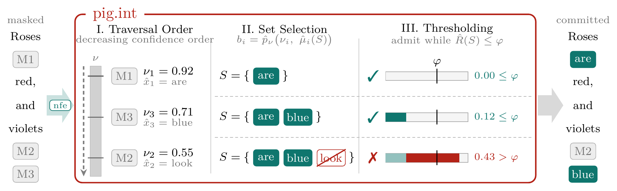
The walk, as drawn in the paper: one forward pass ranks the masked slots by confidence (I); candidates are added with their predicted incremental regret (II) and admitted while the total fits the budget \(\varphi\) (III); the first candidate that does not fit closes the round.
The same walk on a real pass of the decode above:
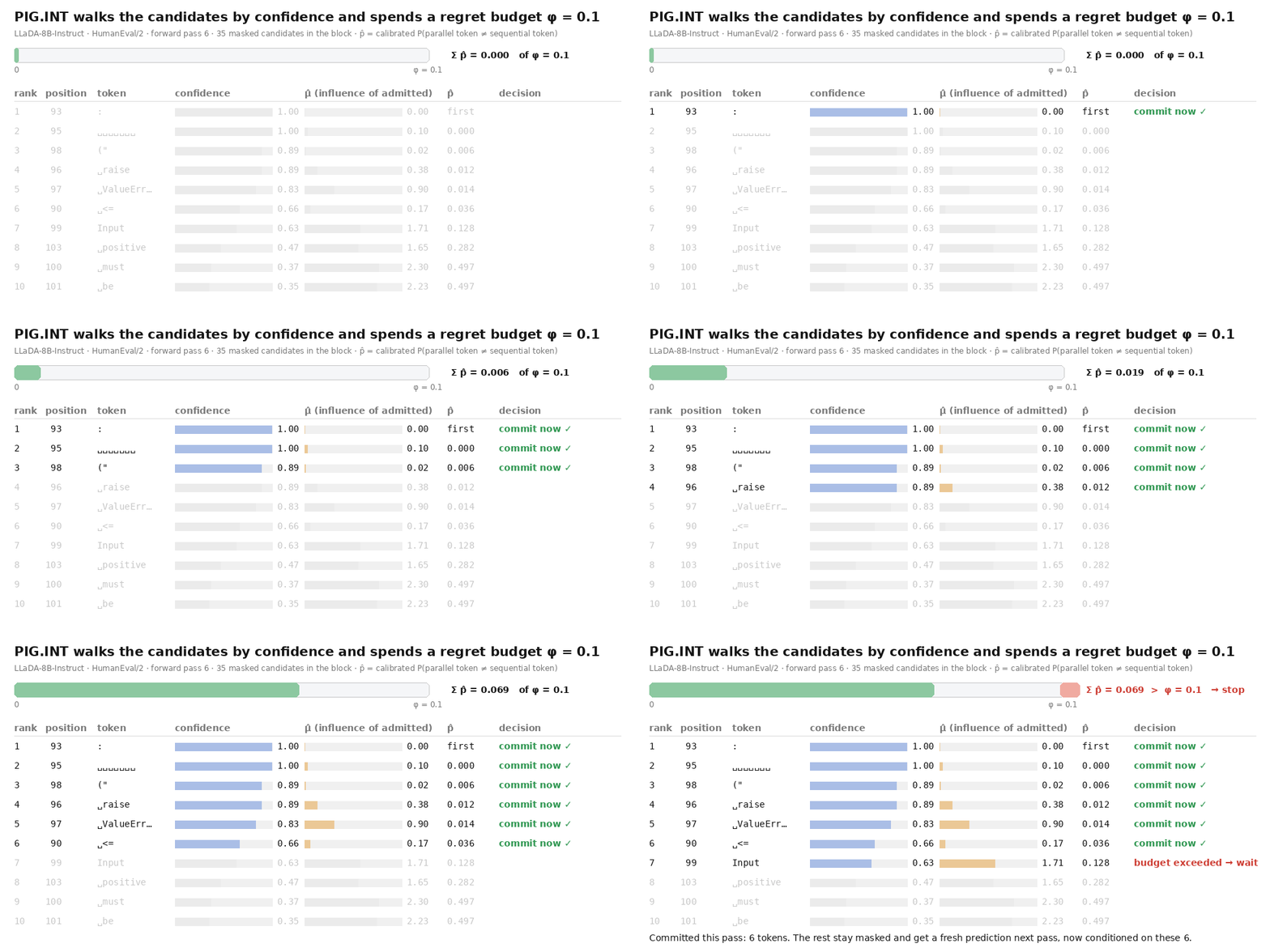
Each admitted token adds its predicted mismatch probability to the budget; the first token that would push the total past \(\varphi\) closes the round, and everything after it waits for a fresh prediction conditioned on what was just committed.
Note what the walk is not doing. It never asks whether two tokens are dependent in the abstract. A pair can be strongly coupled and still both be admitted, if the coupling is the agreeing kind; a weakly coupled token can be refused, if it sits behind many admitted tokens that each nudge it a little.
PIG.EXT: is waiting worth a pass?
PIG.INT controls the error inside the current round. PIG.EXT asks a cross-round question instead: if I stop admitting here and spend one more forward pass, how much predicted regret on the next sixteen candidates disappears because they get to see what I just committed? The round closes when that predicted relief exceeds a budget \(\theta\). Its two slowest operating points additionally refuse tokens below a confidence floor.
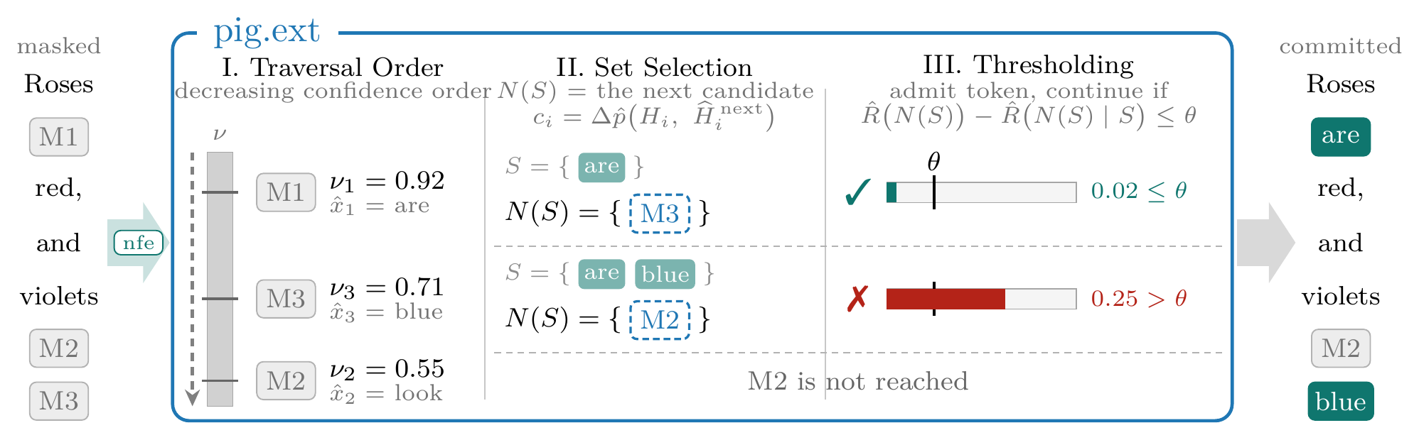
On the same canvas and order, PIG.EXT admits each candidate and then prices the next ones: how much their mismatch risk would drop if it first committed what it has (II). The round continues while that predicted relief stays within \(\theta\) (III): committing “are” changes little, so the walk widens; committing “blue” would flip a later slot, so waiting is worth more than \(\theta\) and the round closes.
The practical effect is that PIG adapts its width to the decode. Where the remaining canvas is flat, both rules commit wide; at the hard spots, where one commitment would reshape the predictions around it, they narrow down.
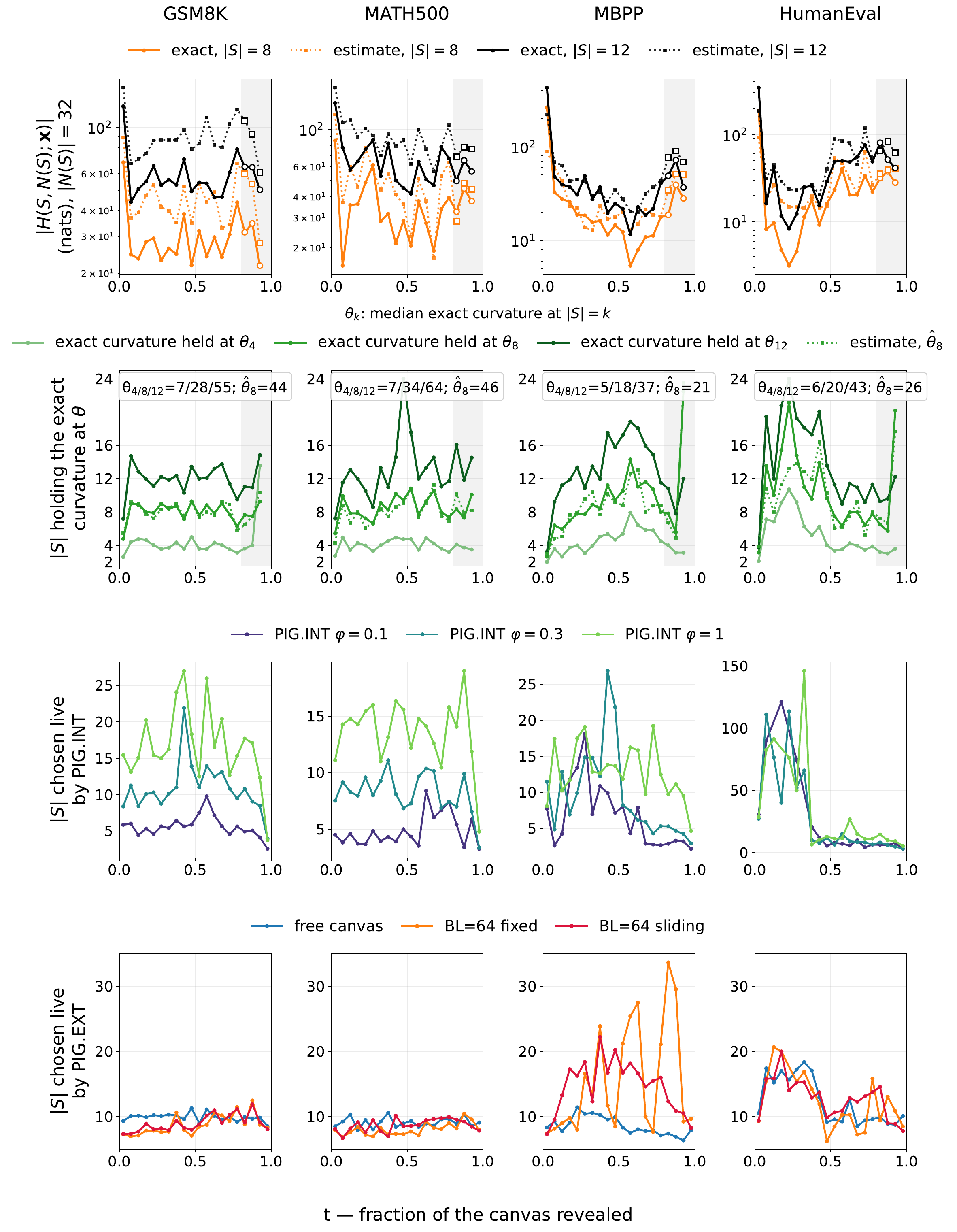
Decoding width and local curvature over the decode on the four benchmarks.
Results
We evaluate LLaDA-8B-Instruct (256-token canvas, Fast-dLLM’s few-shot setup) and Nemotron-Labs-Diffusion-3B-Instruct (2048-token canvas, 0-shot) on GSM8K, MATH-500, MBPP and HumanEval, with greedy commits throughout, and report accuracy against tokens per forward pass (TPF). The baseline is confidence-threshold decoding over the same eligible positions: Fast-dLLM for LLaDA, the native confidence decoder for Nemotron.
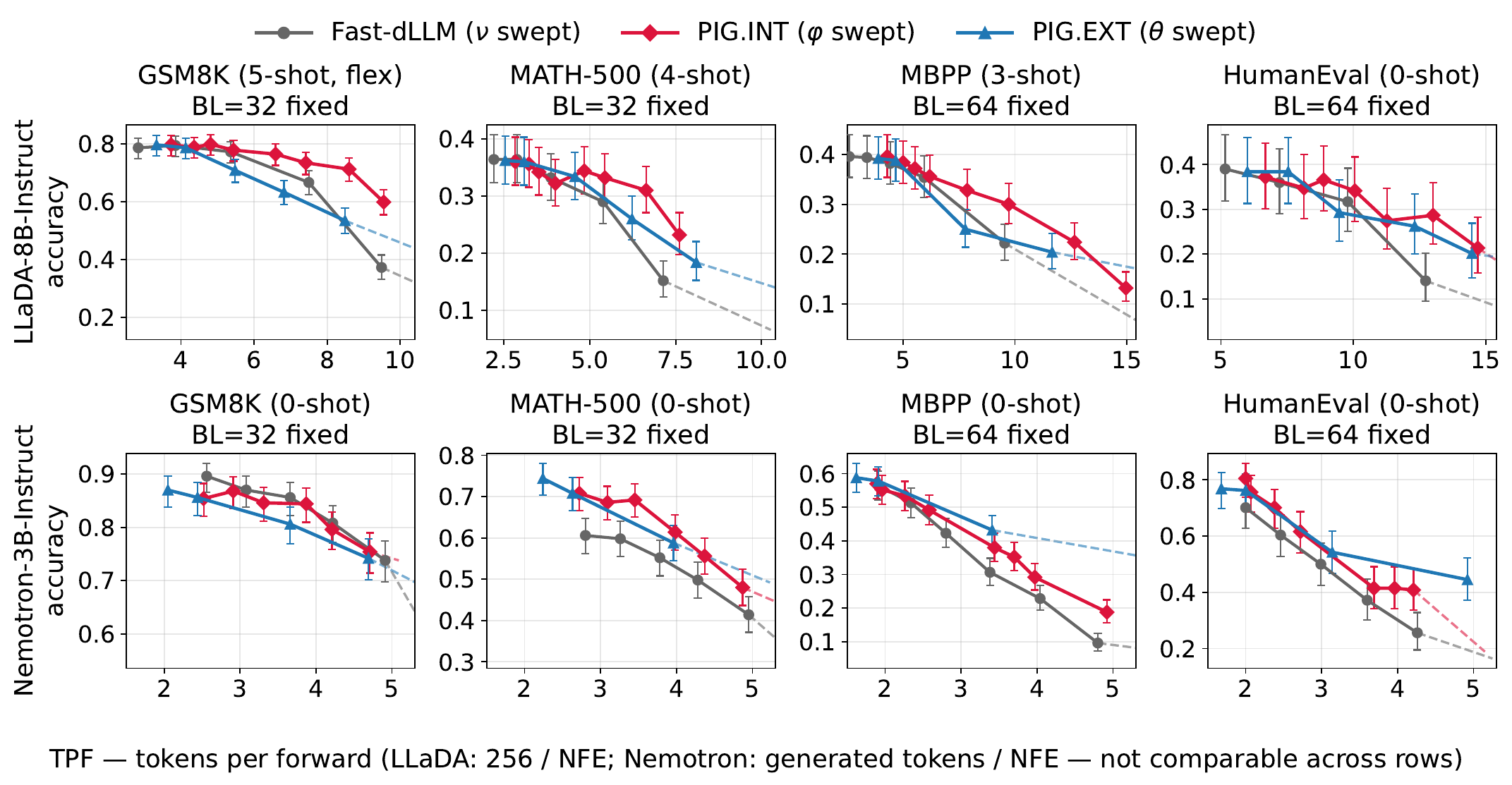
PIG.INT (red) and PIG.EXT (blue) against the confidence baseline (grey) on LLaDA (top) and Nemotron (bottom), fixed blocks. Wilson 95% intervals.
- At matched accuracy, PIG.INT reaches up to 1.7× the TPF of Fast-dLLM on LLaDA and 1.4× of Nemotron’s native decoder.
- At the baseline’s fastest settings, PIG keeps up to 28 more accuracy points. Confidence thresholds collapse when pushed; a regret budget degrades gracefully.
- It transfers. The adapter and the tables are fitted once per backbone on a small mixture (OpenCoder, GSM8K-train, MATH-train, MBPP-train). Reused unchanged on MMLU, a benchmark they never saw, PIG still extends the frontier. Against dependency-guided decoders on LLaDA it reaches up to 4.4× the TPF.
The paper reduces each comparison to one number in two ways. Table 1 asks how much faster PIG runs than each baseline at the baseline’s best accuracy, including the dependency-guided decoders DAPD, EB-Sampler and KLASS. Table 2 asks what accuracy each decoder delivers at a fixed throughput.
| benchmark | our protocol (paired) | their protocol | |||
|---|---|---|---|---|---|
| Fast-dLLM | DAPD-Direct | DAPD-Staged | EB-Sampler | KLASS | |
| PIG.INT: relative TPF increase (accuracy difference in parentheses) | |||||
| GSM8K | 1.15× (+0.0) | 1.77× (+2.0) | 2.62× (+0.6) | 2.51× (+0.5) | 2.71× (+1.0) |
| MATH-500 | 1.13× (−0.2) | 1.65× (+1.0) | 1.82× (+0.6) | 3.38× (+1.2) | 4.38× (+1.4) |
| MBPP | 1.66× (+0.0) | 0.83× (+1.0) | 1.85× (+0.4) | 2.60× (+3.0) | 2.05× (+4.0) |
| HumanEval | 1.29× (−1.8) | 1.46× (+2.4) | 4.28× (+3.1) | 2.88× (+0.0) | 3.90× (−0.6) |
| PIG.EXT: relative TPF increase (accuracy difference in parentheses) | |||||
| GSM8K | 0.85× (−0.6) | 1.04× (+4.4) | 1.91× (+1.4) | 1.47× (+2.9) | 1.59× (+3.4) |
| MATH-500 | 0.87× (+0.6) | 1.00× (+2.4) | 1.57× (+0.8) | 2.84× (+2.0) | 2.97× (+3.8) |
| MBPP | 1.50× (−0.4) | 0.90× (+0.2) | 1.73× (+0.8) | 2.40× (+1.0) | 0.98× (+12.8) |
| HumanEval | 1.46× (−0.6) | 1.10× (+6.7) | 4.06× (+0.6) | 3.25× (+1.2) | 4.40× (+0.6) |
| benchmark | Fast-dLLM | PIG.INT | PIG.EXT | Fast-dLLM | PIG.INT | PIG.EXT |
|---|---|---|---|---|---|---|
| LLaDA-8B-Instruct | interpolated accuracy @ TPF = 10 | interpolated accuracy @ TPF = 15 | ||||
| GSM8K | 51.4 | 70.5 (+19.1) | 56.0 (+4.6) | 25.6 | 34.0 (+8.5) | 39.7 (+14.2) |
| MATH-500 | 14.1 | 25.5 (+11.4) | 20.0 (+5.9) | 9.8 @12.2 | 15.4 @13.4 (–) | 13.7 (–) |
| MBPP | 21.0 | 29.3 (+8.3) | 22.4 (+1.4) | 7.8 | 13.2 @15.0 (+5.3) | 17.5 (+9.7) |
| HumanEval | 30.4 | 34.3 (+3.8) | 28.7 (−1.7) | 9.2 | 20.2 (+11.0) | 19.7 (+10.5) |
| Nemotron-3B-Instruct | interpolated accuracy @ TPF = 3 | interpolated accuracy @ TPF = 5 | ||||
| GSM8K | 86.5 | 83.7 (−2.8) | 83.7 (−2.8) | 76.1 | 76.7 (+0.5) | 75.9 (−0.3) |
| MBPP | 38.3 | 43.7 (+5.5) | 47.2 (+8.9) | 9.1 | 18.8 @4.9 (+9.5) | 36.9 (+27.8) |
| HumanEval | 49.8 | 55.8 (+6.0) | 57.0 (+7.2) | 18.8 | 22.4 (+3.6) | 44.5 @4.9 (+25.0) |
The adapter is also calibrated, not merely correlated: the predicted mismatch rate tracks the realised one along the decoder’s own trajectories.
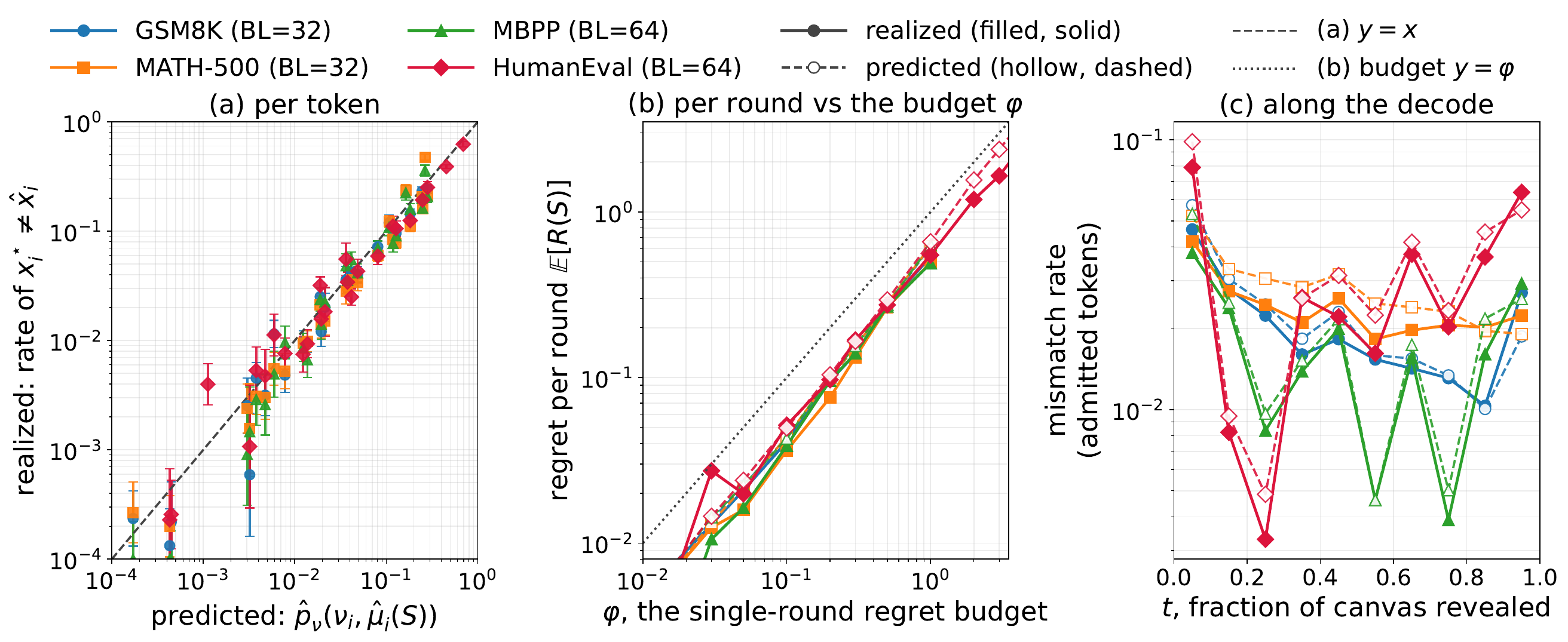
Predicted versus realised mismatch on PIG.INT’s own trajectories (LLaDA).
Try it
Each Hugging Face repository is the whole model: backbone, adapter and tables.
from transformers import AutoModel

model = AutoModel.from_pretrained("UT-IFML/LLaDA-8B-Instruct-PIG", trust_remote_code=True)
out = model.generate("Write a Python function that returns the n-th Fibonacci number.",
                     mode="pig.int", phi=0.1)
print(out.text, out.tpf)
mode="pig.ext", theta=0.5 switches rules, mode="confidence", nu=0.9 gives
the baseline, and geometry/block set which positions are candidates. The
repository has the
evaluation harness that produced every number above.
What it does not do (yet)
The adapter is trained per backbone: for a new model, harvesting the exact finite differences took 26 single-H100 GPU hours and fitting the 2M-parameter adapter about an hour. Commits are greedy; sampling is untouched. The estimator adds about 13 ms per round in our decoder (measured on a shared H100, so an upper bound), which is small next to a forward pass of an 8B model and not nothing for a 3B one. And the padding after the end of a short answer still costs passes on a fixed canvas, as the strip under the first animation shows, for PIG and the baseline alike.
Citation
@article{fruytier2026pig,
  title   = {PIG: Parallel Inconsistency Guidance for Accelerating Diffusion Language Models},
  author  = {Fruytier, Quentin and Xue, Anton and Shakkottai, Sanjay and Sanghavi, Sujay},
  journal = {arXiv preprint arXiv:2610.17375},
  year    = {2026}
}