SIAM Data Mining 2026 · Salt Lake City

Sculpting the Latent Space

Disentanglement with WAE-MMD and Programmable Priors

Quentin Fruytier¹ · Akshay Malhotra² · Shahab Hamidi-Rad² · Aditya Sant² · Aryan Mokhtari¹ · Sujay Sanghavi¹

¹ The University of Texas at Austin · ² InterDigital Communications, AI Lab

The goal

Disentanglement asks for two different things

Mutually independent latents

No latent unit can be predicted from the others, over the whole dataset.

Semantically meaningful latents

Each unit lines up with a real factor: shape, scale, position, colour.

Without supervision, (2) is not identifiable: many independent representations fit the same data. Unsupervised methods can only aim at (1). We measure (1), enforce it, and then inject (2) through the prior.

Hyvärinen & Pajunen 1999; Locatello et al. 2019, 2020; Khemakhem et al. 2020

The failure

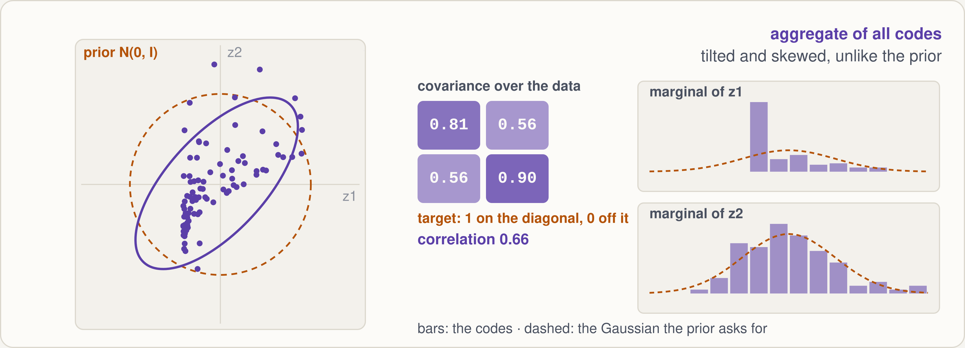
A per-sample KL does not shape the aggregate

Schematic in two dimensions · the next slide shows the same failure measured on MNIST

Final frame: the aggregate of all codes is tilted and skewed unlike the N(0, I) prior; covariance 0.81, 0.56, 0.56, 0.90, correlation 0.66; marginals of z1 and z2 depart from the Gaussian

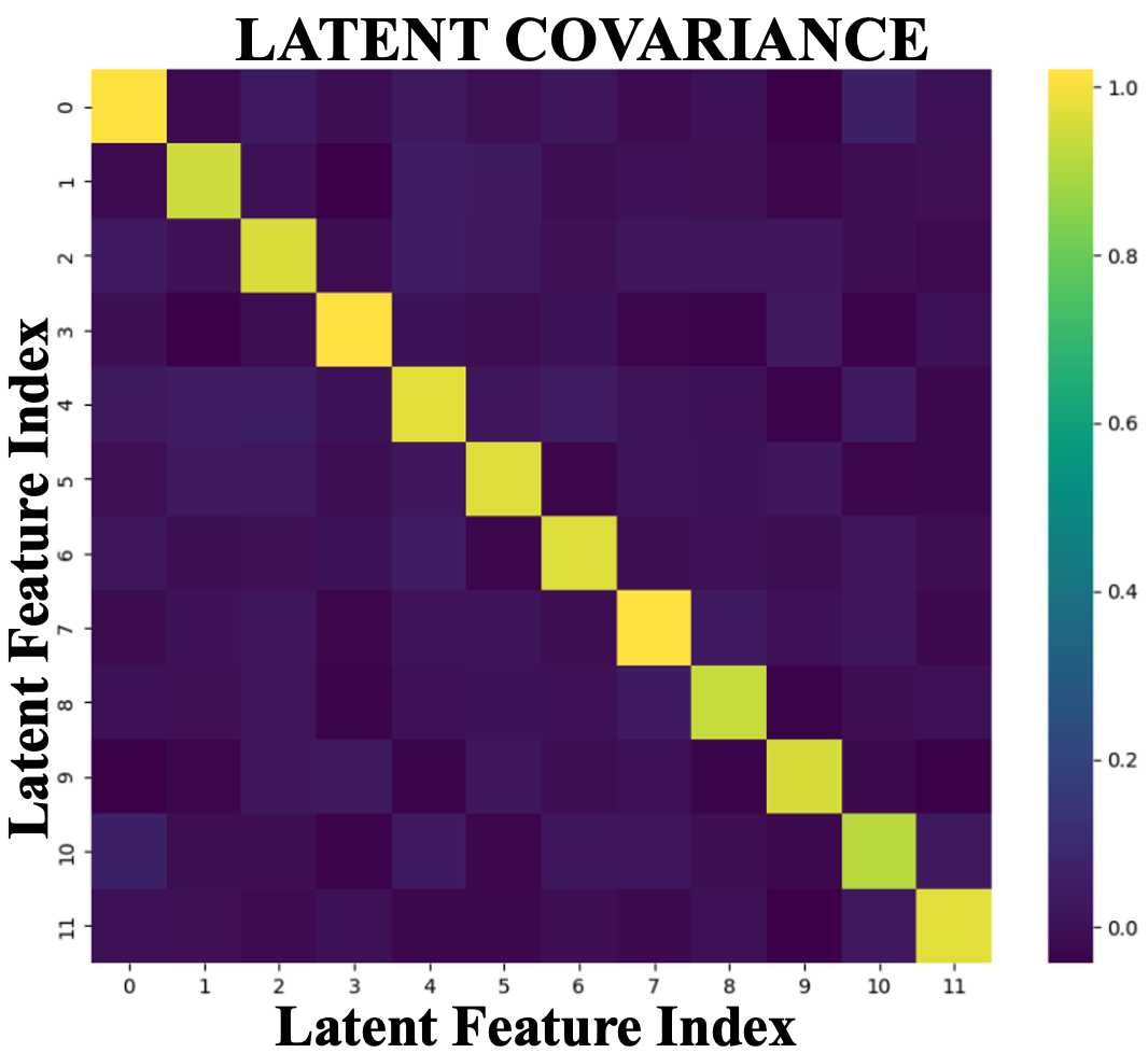
The evidence · MNIST, 12 latent dimensions

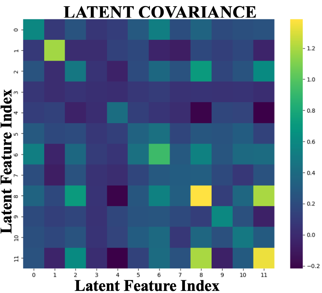
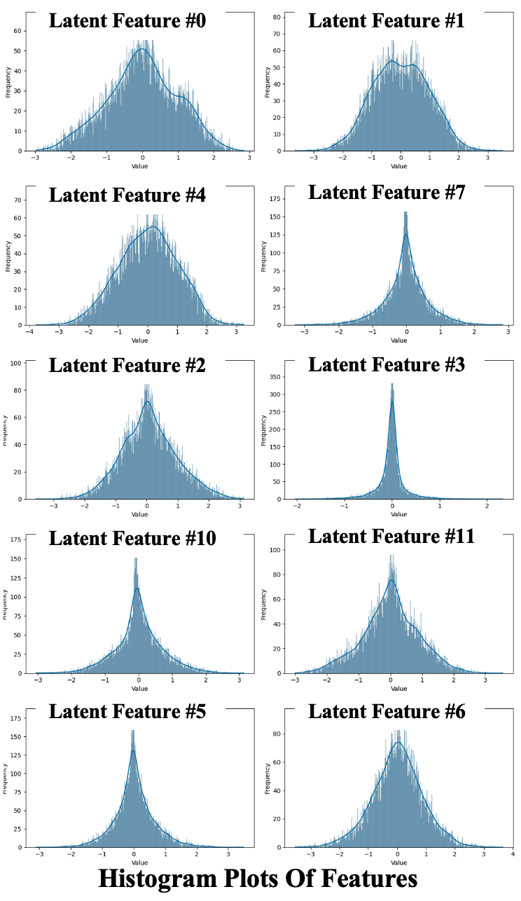
Only the MMD model matches the prior

Standard VAE

β-VAE (β = 4)

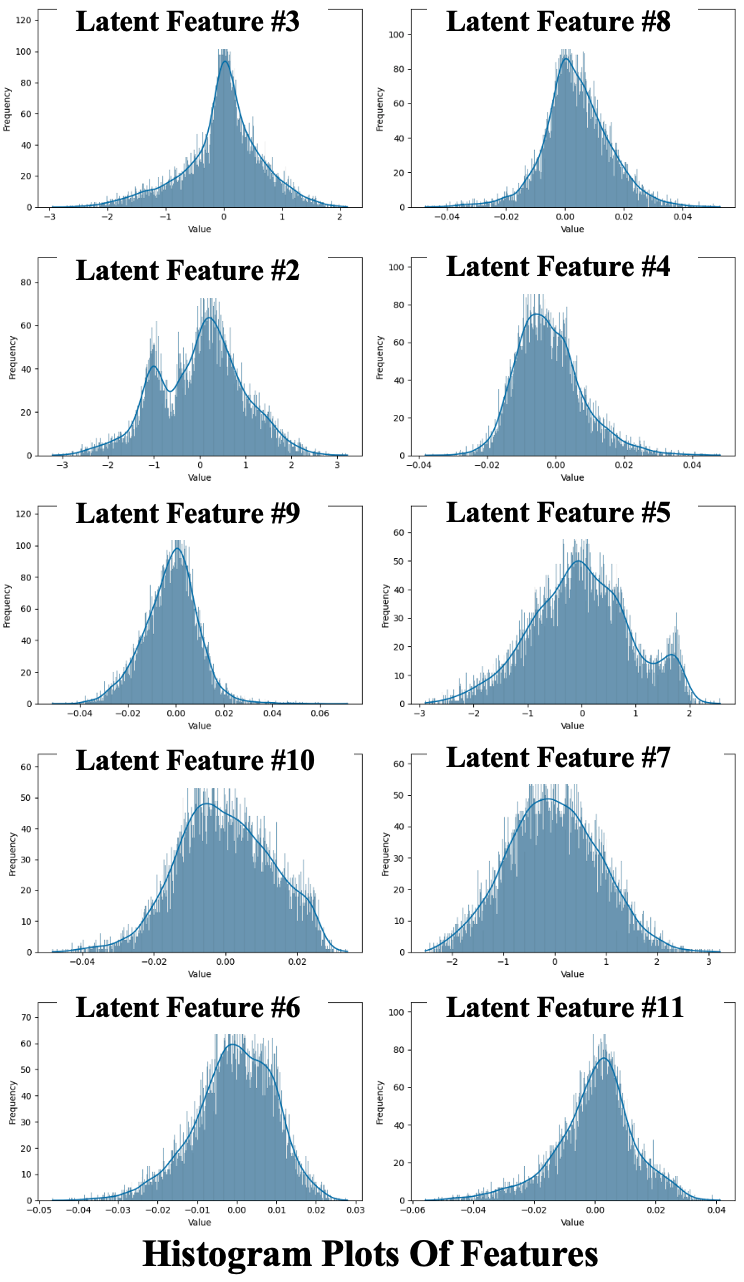
SWAE-MMD (ours)

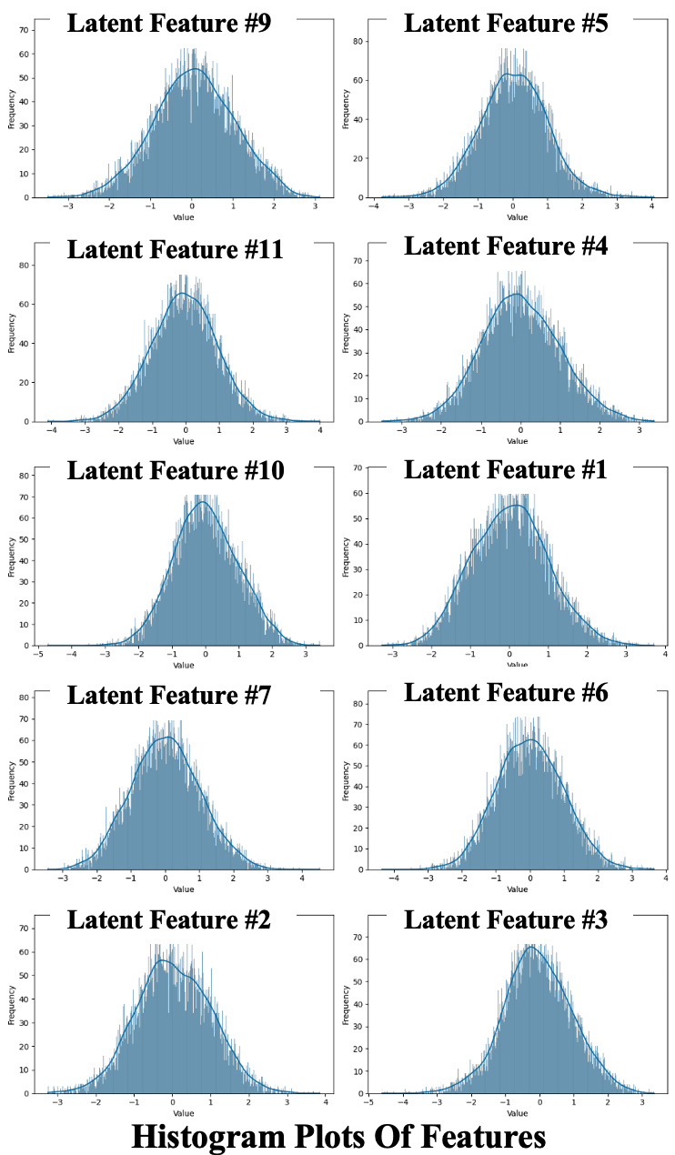
SWAE-MMD latent covariance over MNIST, diagonal

SWAE-MMD latent marginal histograms, Gaussian

AE + batch KL

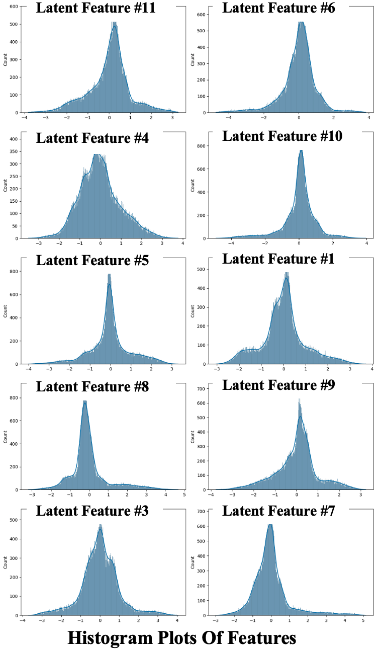
Autoencoder with batch-wise KL: latent covariance over MNIST

Autoencoder with batch-wise KL: latent marginal histograms

Standard AE

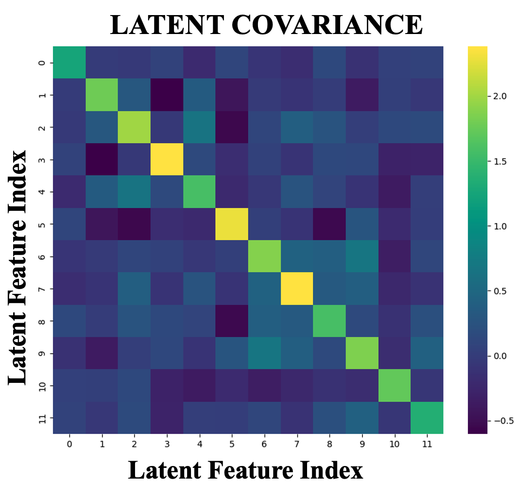
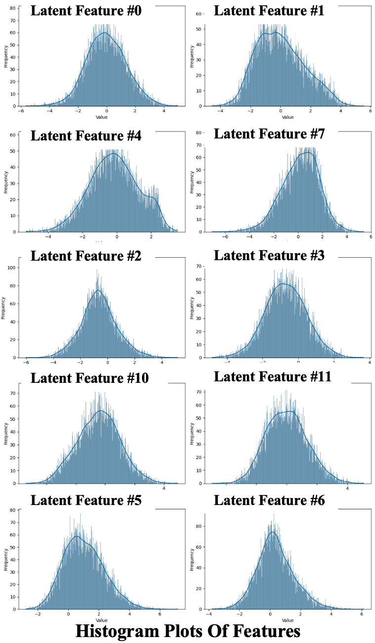
Standard autoencoder latent covariance over MNIST

Standard autoencoder latent marginal histograms

Top: covariance of the latents over the dataset · bottom: their marginals · batch KL fixes two moments, yet its LPS is 0.97

Measuring it without labels

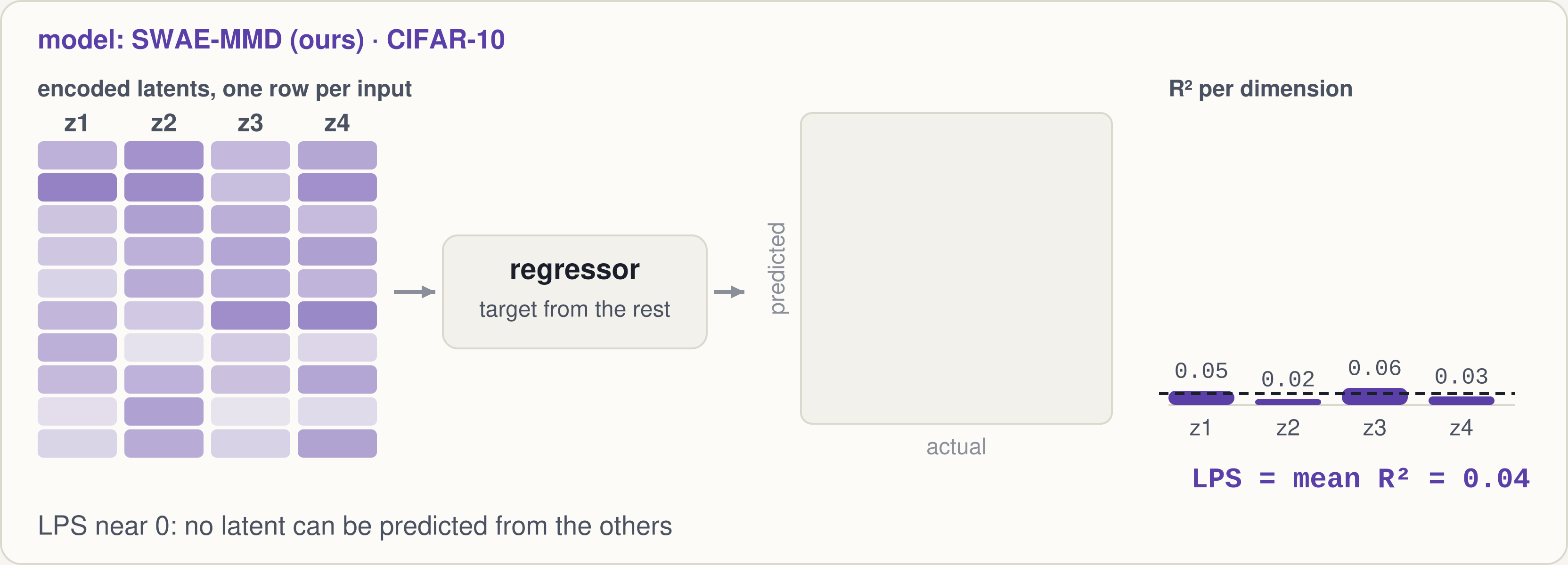
The Latent Predictability Score

4 of 64 dimensions shown; per-dimension R² illustrative · LPS values are Table 1’s CIFAR-10 numbers (LightGBM regressor)

Final frame: for SWAE-MMD on CIFAR-10 every per-dimension R squared is near zero and LPS = mean R squared = 0.04; no latent can be predicted from the others

Why the score is safe to trust

LPS can only underestimate entanglement

R² of any regressor ≤ η², the share of a latent’s variance the others truly explain

No regressor beats the conditional mean. So an LPS of 0.5 proves that at least half of the latent information is entangled, whatever the ground-truth factors are: a rejection test that needs no labels.

The fix · SWAE-MMD

Match the aggregate posterior to prior samples

maximise E[ log q(x) ] − λ · MMD²( q(z), p(z) )

reconstruct the input, and make the distribution of all codes match the prior, using only samples of the prior

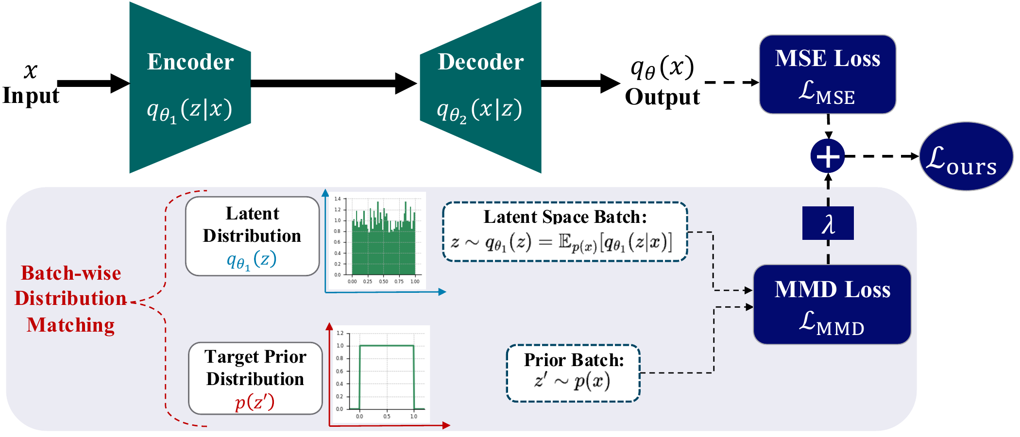
Architecture: encoder and decoder with an MSE loss, plus an MMD loss between the latent batch and a batch sampled from the target prior

The regularizer acts on the batch, not on each sample: it sees the whole aggregate shape.

It needs no density for p(z), only a way to sample it. That is what makes the prior programmable.

A Wasserstein autoencoder variant (Tolstikhin et al. 2018) used for representation engineering · batch 512, λ = 0.3

Sculpting, one batch at a time

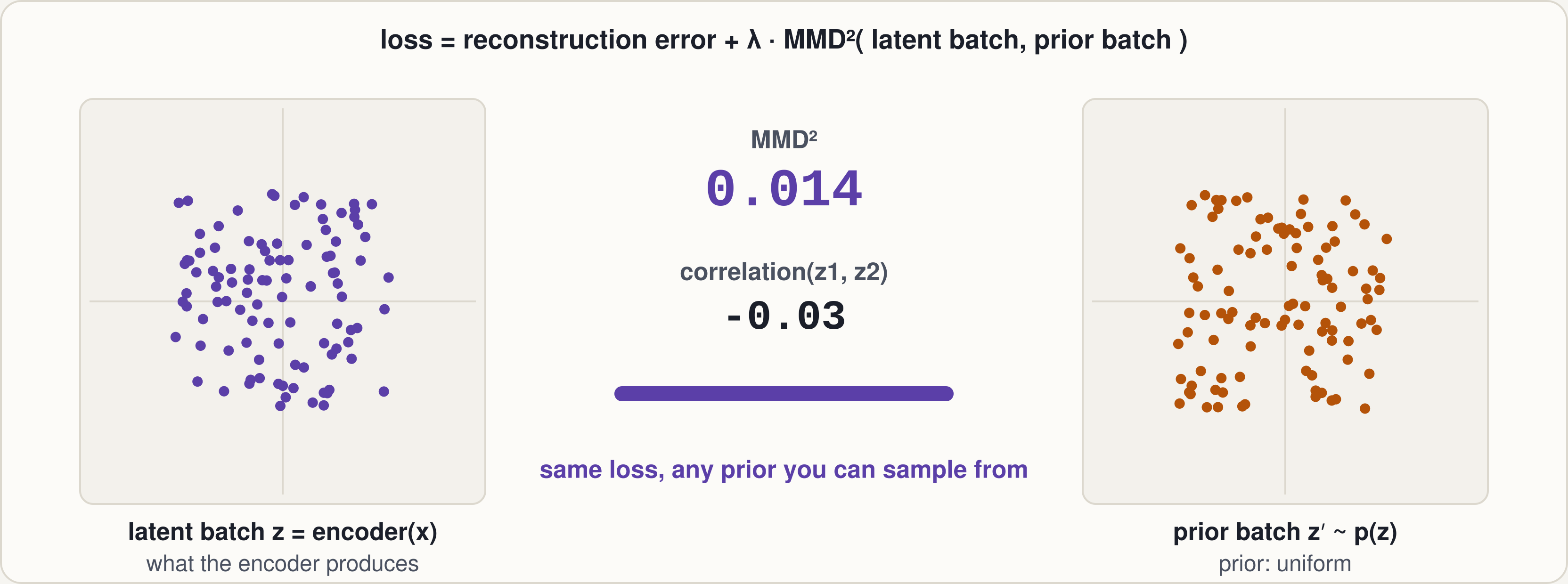
MMD pulls the codes onto any prior

Two latent dimensions, schematic training · MMD² and the correlation are computed live from the points shown (Gaussian kernel)

Final frame: after swapping to a uniform prior the latent batch matches it, MMD squared 0.014 and correlation -0.03; same loss, any prior you can sample from

Results · 8 datasets

70% less entanglement than the next best method

LPS (mean R², lower = more independent); latent size in brackets

model	ImageNet [64]	CIFAR-10 [64]	MNIST [12]	dSprites [5]	XY [2]	XYC [3]	XYCS [4]	CelebA [32]
SWAE-MMD (ours)	0.03	0.04	0.22	0.04	−0.05	−0.01	0.11	0.08
FactorVAE (γ = 10)	0.44	0.63	0.27	0.08	−0.04	0.00	0.17	0.07
NashAE	0.56	0.17	0.22	0.10	−0.07	0.14	0.37	0.36
β-TCVAE (β = 4)	0.79	0.89	0.84	0.22	−0.04	−0.01	0.17	0.59
β-VAE (β = 4)	0.73	0.85	0.90	0.52	−0.05	0.00	0.28	0.53
DGAE	0.77	0.69	0.63	0.56	0.25	0.50	0.59	0.48

Averaged over the 8 datasets, LPS falls by 70% against FactorVAE, with reconstruction as good or better (CIFAR-10: −15.61 dB NMSE vs −12.49 dB).

Table 1 of the paper · bold = best in column · R² slightly below 0 on held-out data means nothing is predictable

Results · CIFAR-10

Independence holds as the latent space grows

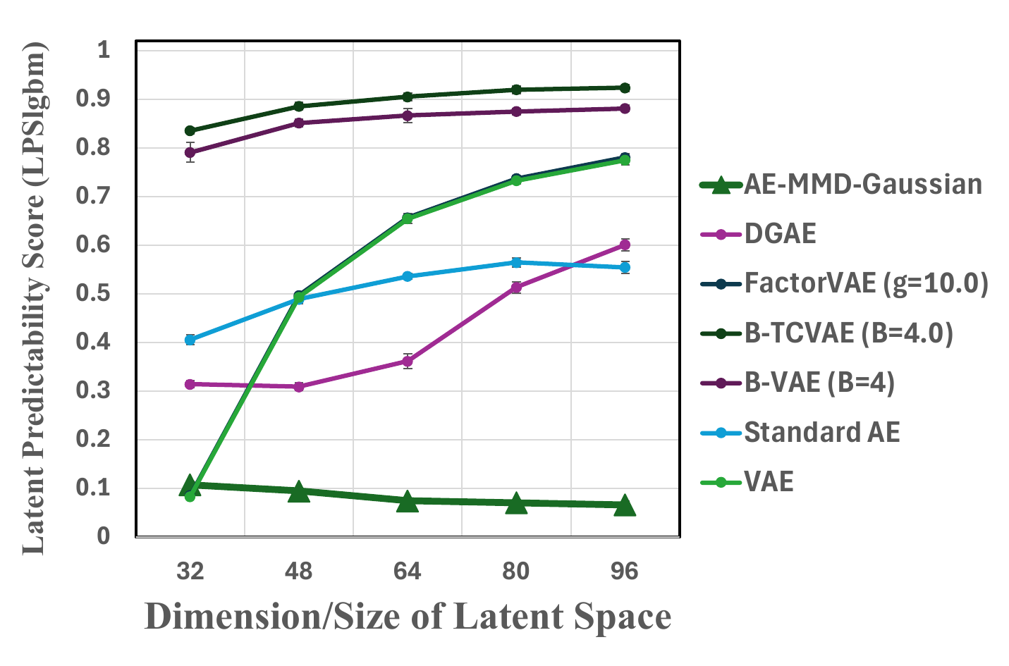
LPS against latent dimension 32 to 96 on CIFAR-10: AE-MMD-Gaussian stays near 0.1 while the baselines rise toward 0.6 to 0.9

Flat in the latent size

From 32 to 96 dimensions the MMD model stays low, at about 0.1 or below, while most baselines grow more entangled.

Insensitive to its knobs

Batch 64 to 2048, λ from 0.1 to 5, 1 to 5 kernel bandwidths: only small changes in LPS and reconstruction.

LPS with a LightGBM regressor; lower is better · ablations in the paper’s appendix

Programmable prior 1 · semantic alignment

A few pseudo-labels lock latents to real factors

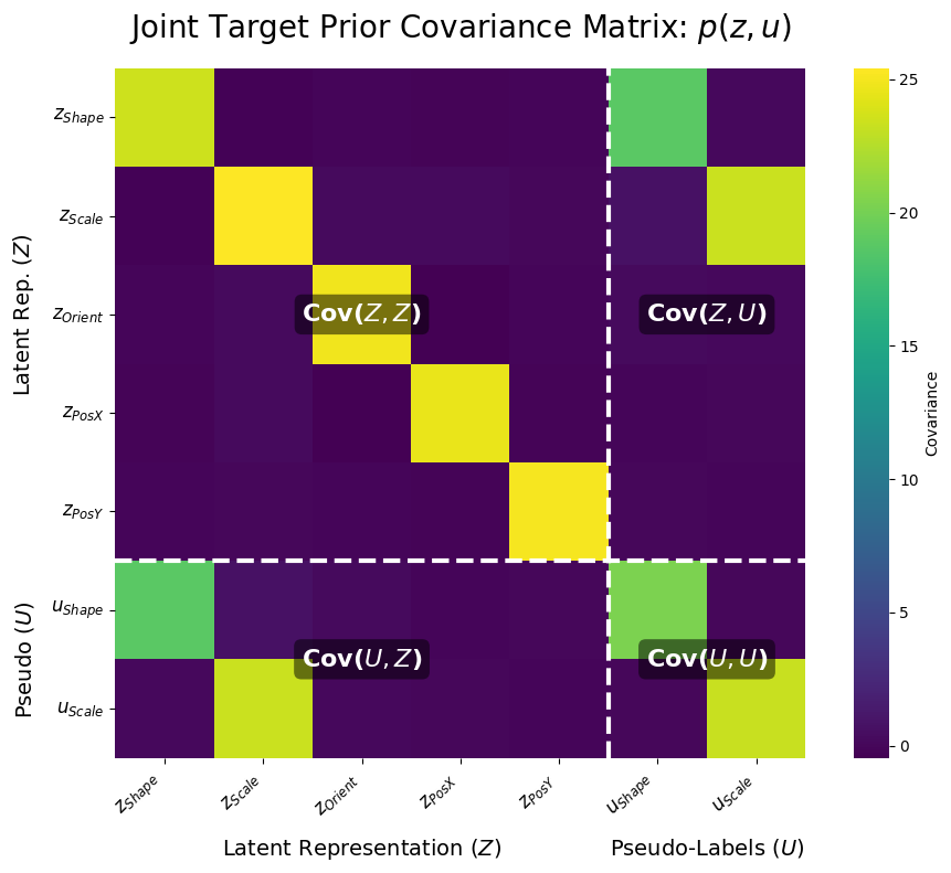
The prior becomes a joint over (z, f(u)) whose first k latents equal the pseudo-labels; MMD on the joint ties those latents to the labels and keeps the rest independent.

target joint

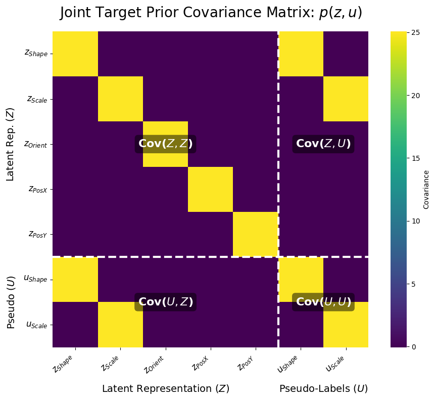
learned joint

DCI disentanglement vs pseudo-labels aligned

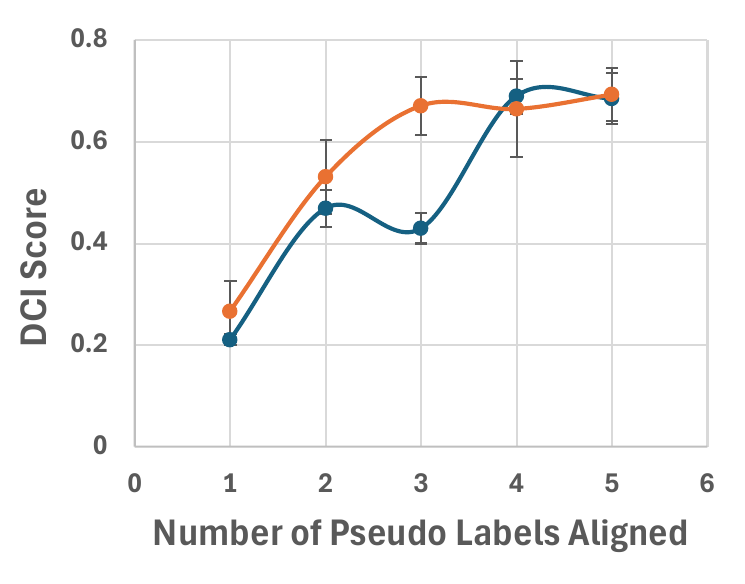
DCI score rising from about 0.2 with one pseudo-label to about 0.7 with four or five, for Gaussian and uniform priors

dSprites · DCI peaks at 3 of 5 factors (uniform prior, orange) and 4 of 5 (Gaussian, blue); reported Ada-GVAE and Ada-ML-VAE stay below 0.5

Programmable prior 2 · compression

Shape the codes to fit the quantizer

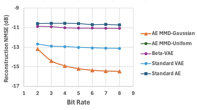
Train with the quantizer in the loop and a prior equal to the distribution the quantizer assumes, Gaussian or uniform.

Gaussian quantizer · CIFAR-10

Reconstruction NMSE against bit rate with a Gaussian quantizer on CIFAR-10: the MMD-Gaussian model is several dB lower than Beta-VAE, Standard VAE and Standard AE

Uniform quantizer · CIFAR-10

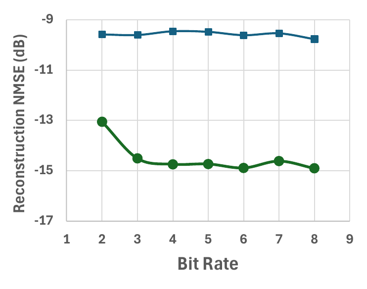
Reconstruction NMSE against bit rate with a uniform quantizer on CIFAR-10: the MMD model in green is several dB below the baseline

2–7 dB lower reconstruction error at 2 to 8 bits per dimension, with no post-training vector quantization or entropy coding.

Reconstruction NMSE in dB, lower is better · green: the MMD model matched to the quantizer

Programmable prior 3 · any distribution you can sample

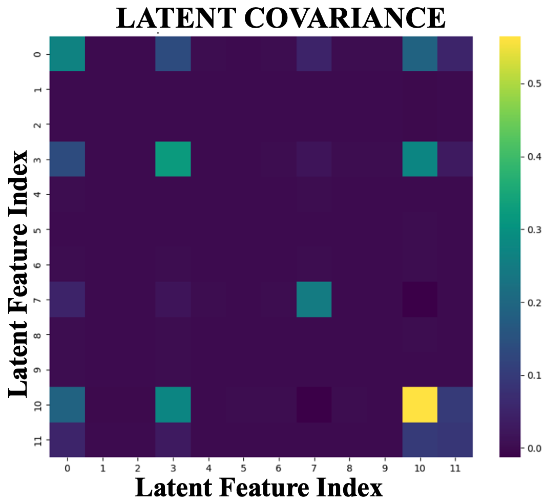
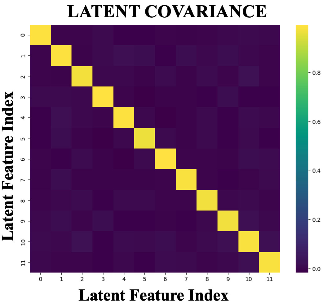
MMD can copy another model’s latent space

teacher: a standard AE’s codes, used as the prior

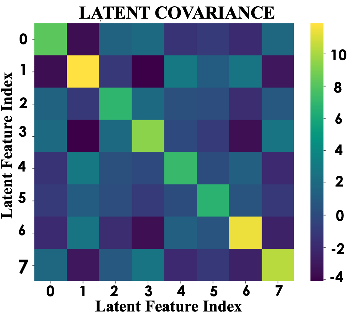
Latent covariance of a standard autoencoder on MNIST, entangled

student: trained with MMD to match them

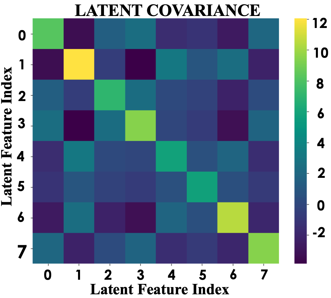
Latent covariance of the MMD student on MNIST, nearly identical to the teacher

An entangled, co-dependent geometry that no closed-form KL target could express.

Covariance and marginals come out nearly identical.

MNIST, latent covariance over the dataset · paper appendix, latent copying experiment

Takeaways

The prior is an engineering tool, not a fixed assumption

A label-free test

LPS lower-bounds entanglement and exposes the VAE-style failure.

A regularizer that works

MMD on the aggregate posterior: 70% less entanglement, reconstruction kept.

One loss, many priors

Semantic alignment, quantizer matching and latent copying.

Joint work with

Akshay Malhotra

InterDigital

Shahab Hamidi-Rad

InterDigital

Aditya Sant

InterDigital

Aryan Mokhtari

UT Austin

Sujay Sanghavi

UT Austin

arxiv.org/abs/2510.11953 · github.com/Quentin-Fruytier/Sculpting-Latent-Spaces-With-MMD

Work done at InterDigital AI Lab with the University of Texas at Austin · thank you